Welcome to Meggie (1.3) user documentation

Getting started (video tutorial)

In this video, meggie is opened for the first time and simple single-subject analysis with sample_audvis_raw.fif is done.

Setting custom channel groups (video tutorial)

In this video, a channel group for the highest point of the head (i.e vertex) is added to the channel groups.

Simple multi-subject analysis with EEG resting state data

In this tutorial, we use 180 second long resting state EEG datasets, with first 90 seconds eyes open and last 90 seconds eyes closed, from 28 subjects, to compare spectral difference between eyes open and eyes closed conditions. The dataset is not available for public, but the tutorial should still make the principles clear.

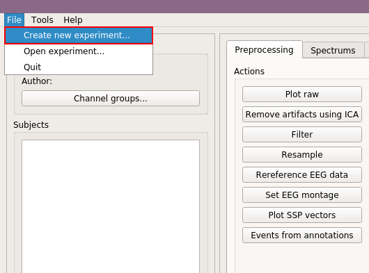
Start by selecting "Create new Experiment" under "File" menu.

Fill experiment details, here we use "EOEC" for experiment name, and "Internet" for author, and then click "Ok."

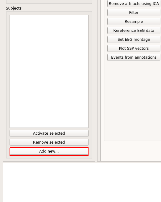
To add the datasets (we are gonna call them subjects from now on), click "Add new..."

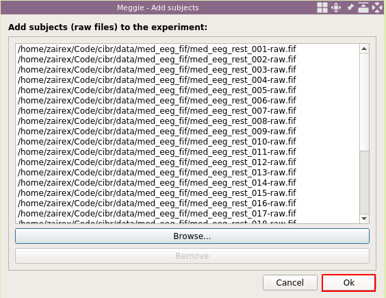
Then click "Browse..", and select the files. You can add them all at once, or one at a time. If one at a time, then use "Browse.." again until all paths are in the list.

Then click "Ok."

Next, select the name of the first (or some other) subject, and click "Activate selected."

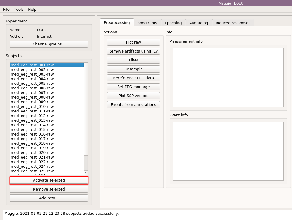
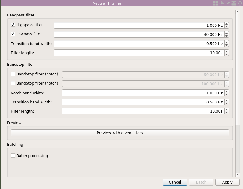
Some information about the subject appears on the "Measurement info" box on the right. We are going to filter the data from 1Hz to 40Hz, resample it to 100Hz and set a standard montage. Standard montage is set because, in this case, the raw files do not contain channel location information. We need the channel location information because we are going to compute channel averages. Select "Filter."

We use the default settings. However, we will use the batch processing option to filter all the subjects in one go. Select "Batch processing."

Click "Select all."

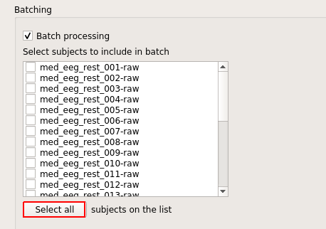
And click "Batch."

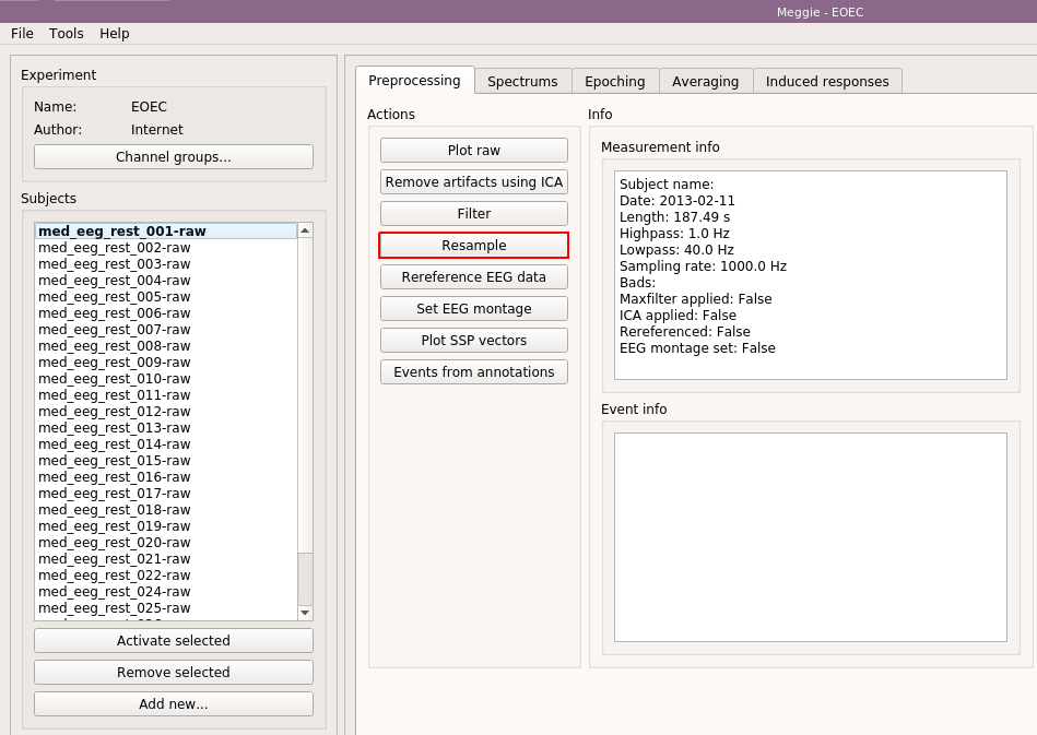
In the measurement info box, you can now see the "Highpass" and "Lowpass" elements to have changed to new values. Next, click "Resample."

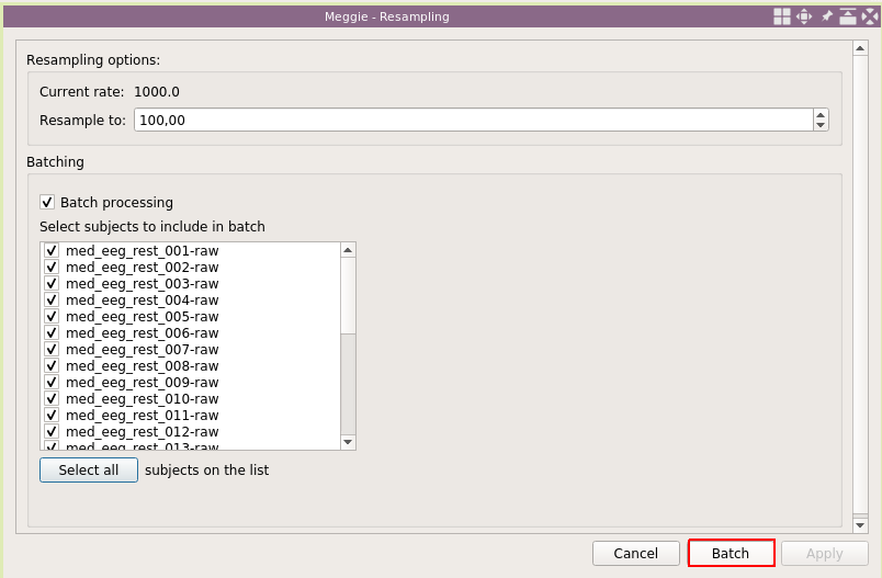
Again, use defaults, and select "Batch processing."

Click "Select all."

And click "Batch."

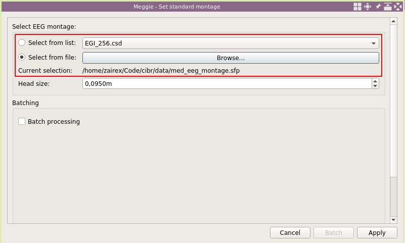
"Sampling rate" in the measurement info box has updated. Next click "Set EEG montage."

The list has many good options for montages (the ones shipped with MNE-Python), and often one can just use one of them. However, with the cap we had, none of the montages in the list was quite right. Thus we had to use a custom montage file

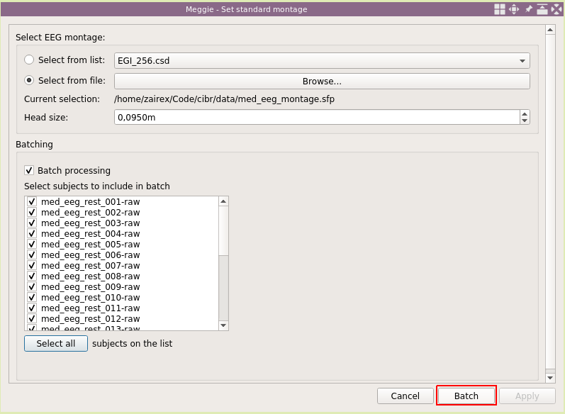
Once again, select "Batch processing."

Click "Select all."

And click "Batch."

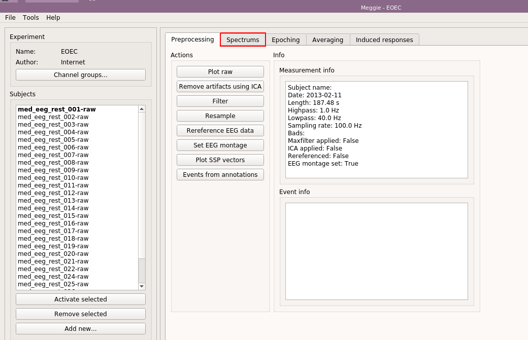
Our purpose is to create a power spectral density of the eyes open and eyes closed conditions, and have them overlayed in a plot. Thus, we move to the "Spectrums" tab, by clicking on it.

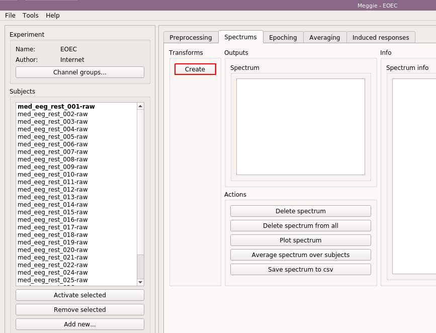
Click "Create spectrum."

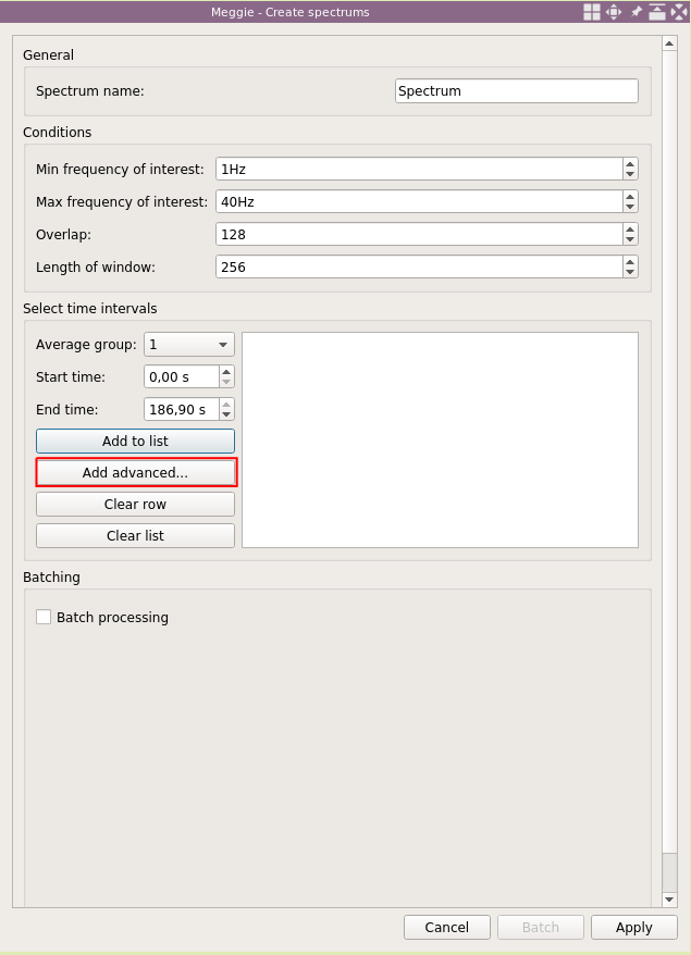
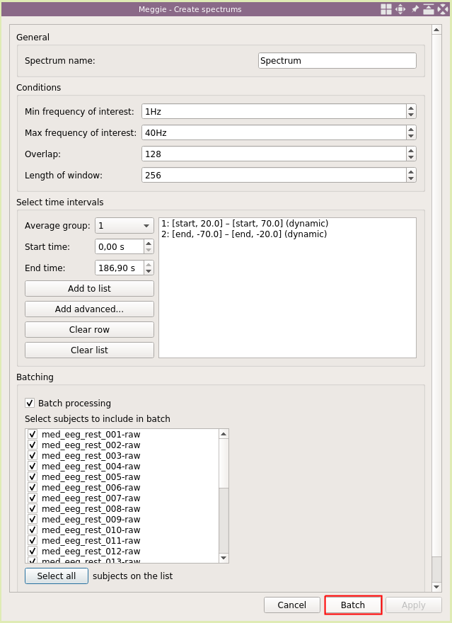
We will use the default settings for naming and window sizes. However, we need to tell the spectrum computation the location of eyes open and eyes closed conditions. As the length of recording is almost the same (180s) for each subjects, we could use static time intervals (using "Add to list"). However, in real life, the lengths can be quite variable, and we will show the dynamic way. Click "Add advanced.."

We will use average group "1" for eyes open condition. Select "Use start of recording" and set offset to be "20s" in the "Starting points" (higher) box. Then select "Use start of recording" and set offset to "70s" in the "Ending points" (lower) box. This way can we set an interval relative to some point (this time it is the beginning of the recording, and we would have gotten identical results by using the static time interval.) Click "Add."

Dynamic interval has appeared in the box of time intervals. Click "Add advanced.." again.

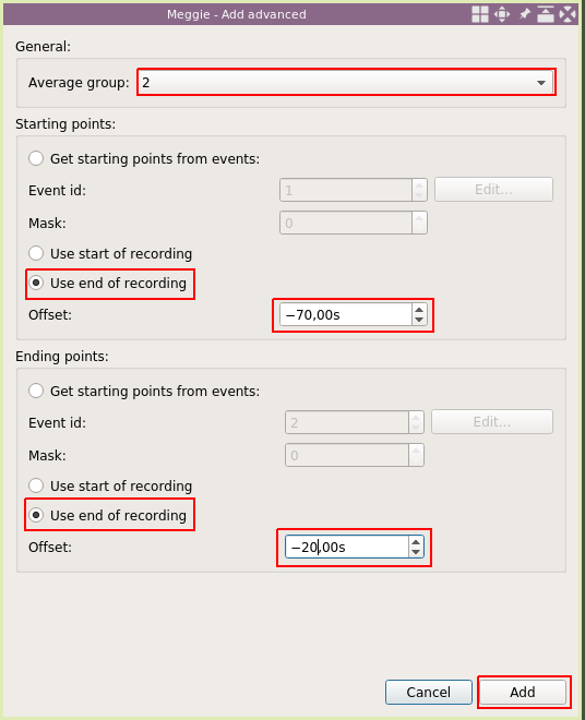
This time, set average group to "2" as we are adding interval for the eyes closed condition. Select "Use end of recording" with "-70s" offset for "Starting points" and select "Use end of recording" with "-20s" offset for "Ending points." This interval will be relative to the end of recording, and could not have been added using the static intervals. Click "Add."

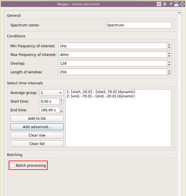
The list now has two items, the first describing the location of the eyes open condition, and the second describing the location of the eyes closed condition. The idea for 20s and 70s is to avoid the edges of the recording and the transition between conditions. Next, select "Batch processing" to create the spectrums for every subject in one go.

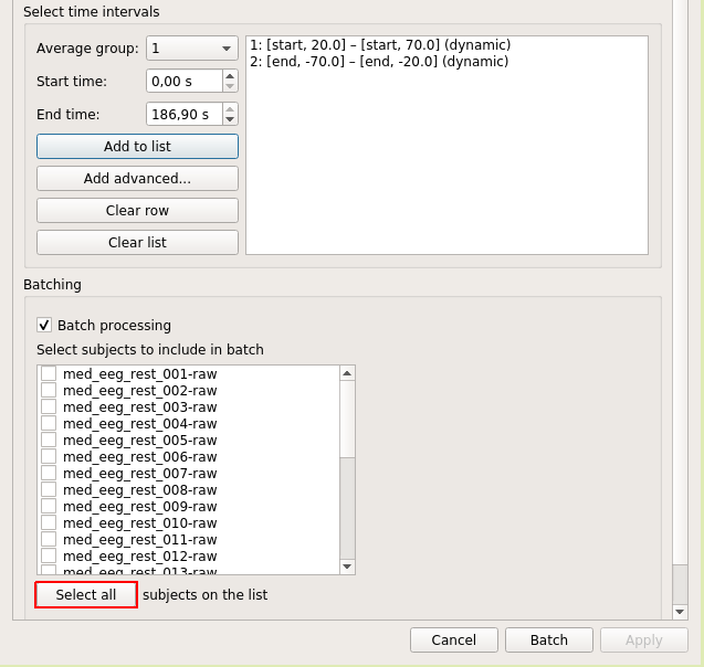
Click "Select all."

Click "Batch."

As we see, an item named "Spectrum" has appeared in the Spectrum box. Select it by clicking

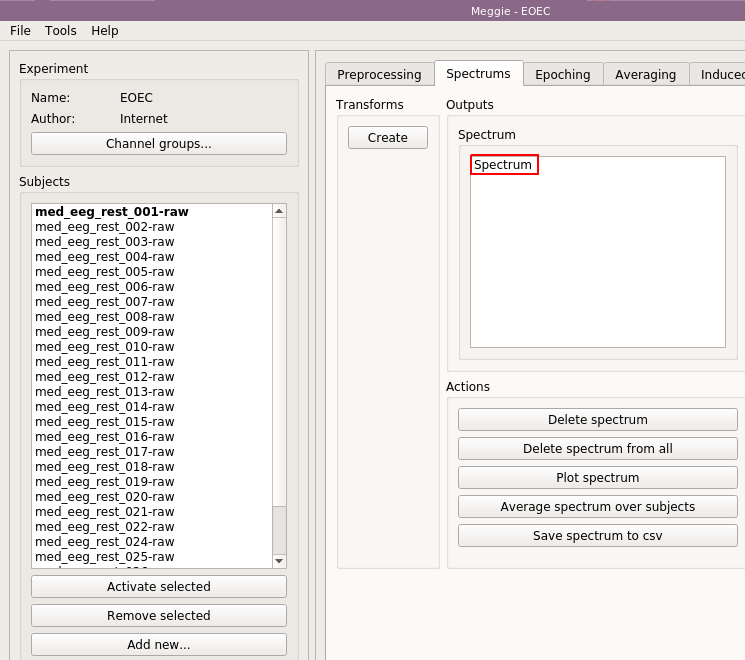
Some information on the spectrum will appear in the "Spectrum info" box. As it was created using batching, similar item with same name (but different data) is now present for other subjects too and could be seen by activating other subject. Next, however, we are going to average over all these spectrum items present in all subjects. Select "Average spectrum over subjects.

We will use the default settings. Checkboxes indicate which subjects to include in the group average, and the numbers allow to separate them into different groups. We want to select all of them, and want all of them in the same group, so just click "Accept."

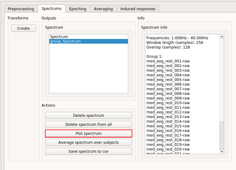
Next, we are going to visualize the results. Select "group_Spectrum" from the "Spectrum" box by clicking.

Information on the item appears on the "Spectrum info" box. In contrast to the "Spectrum" item, which is present for all subjects, "group_Spectrum" item is, even though it is based on the data from all subjects, only stored under the active subject. Click "Plot spectrum.

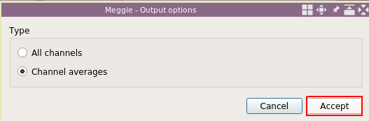
Select "Channel averages". By default, channel averages use standard groups of channels from MNE-Python, that is, "Left-frontal", "Right-frontal", "Left-occipital", "Right-occipital", "Left-parietal", "Right-parietal", "Left-temporal" and "Right-temporal." The standard groups are computed using the channel locations, and that is why it was necessary to set the montages. One can also create custom groups of channels by clicking "Channel groups.." in the left panel of main window just under the "Name" and "Author" fields.

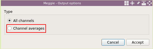
Then click "Accept."

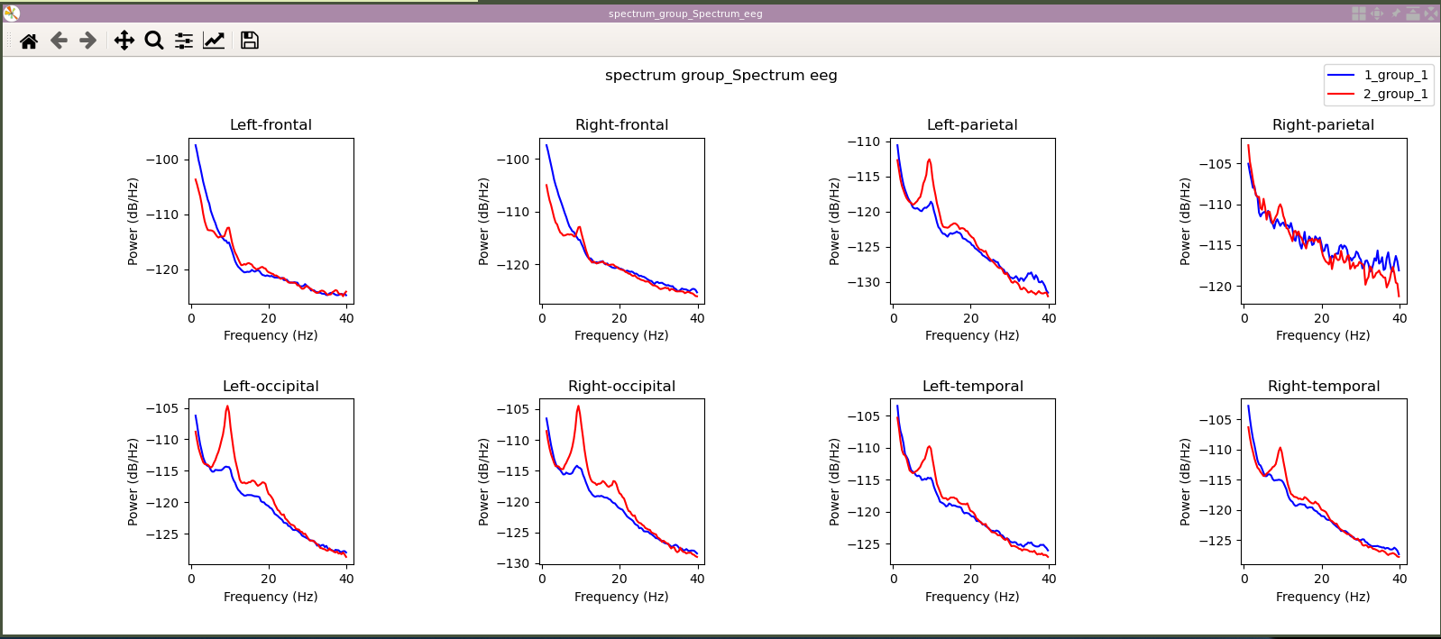
An matplotlib figure is created and shown containing all the channel averages. So, for example, the bottom left one shows an average over all subjects and all channels grouped under "Left-occipital" name. We note that in this case, the occipital alpha around 10Hz is much higher in the eyes closed condition ("2_group_1", first number being the number selected when creating the spectrums and the second number being the number selected when averaging over subjects)) than the eyes open condition ("1_group_1"). You can close the figure.

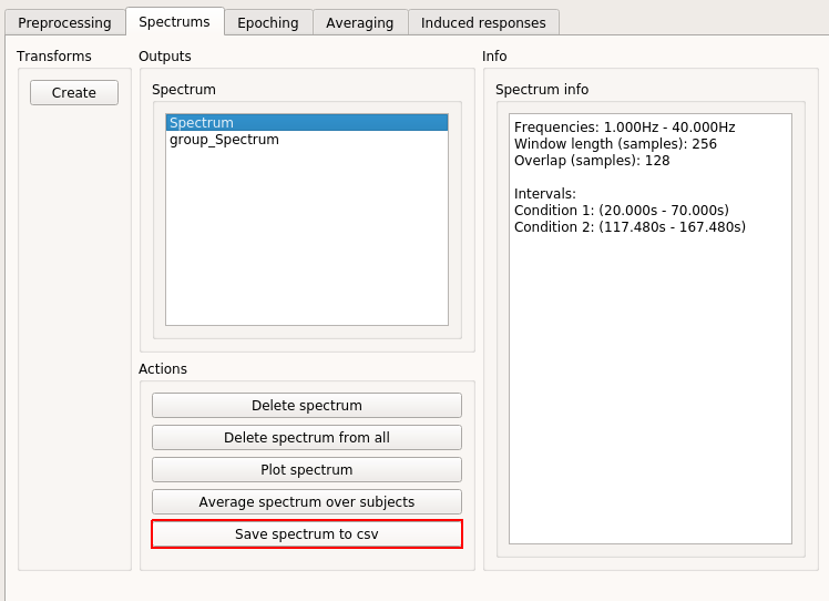
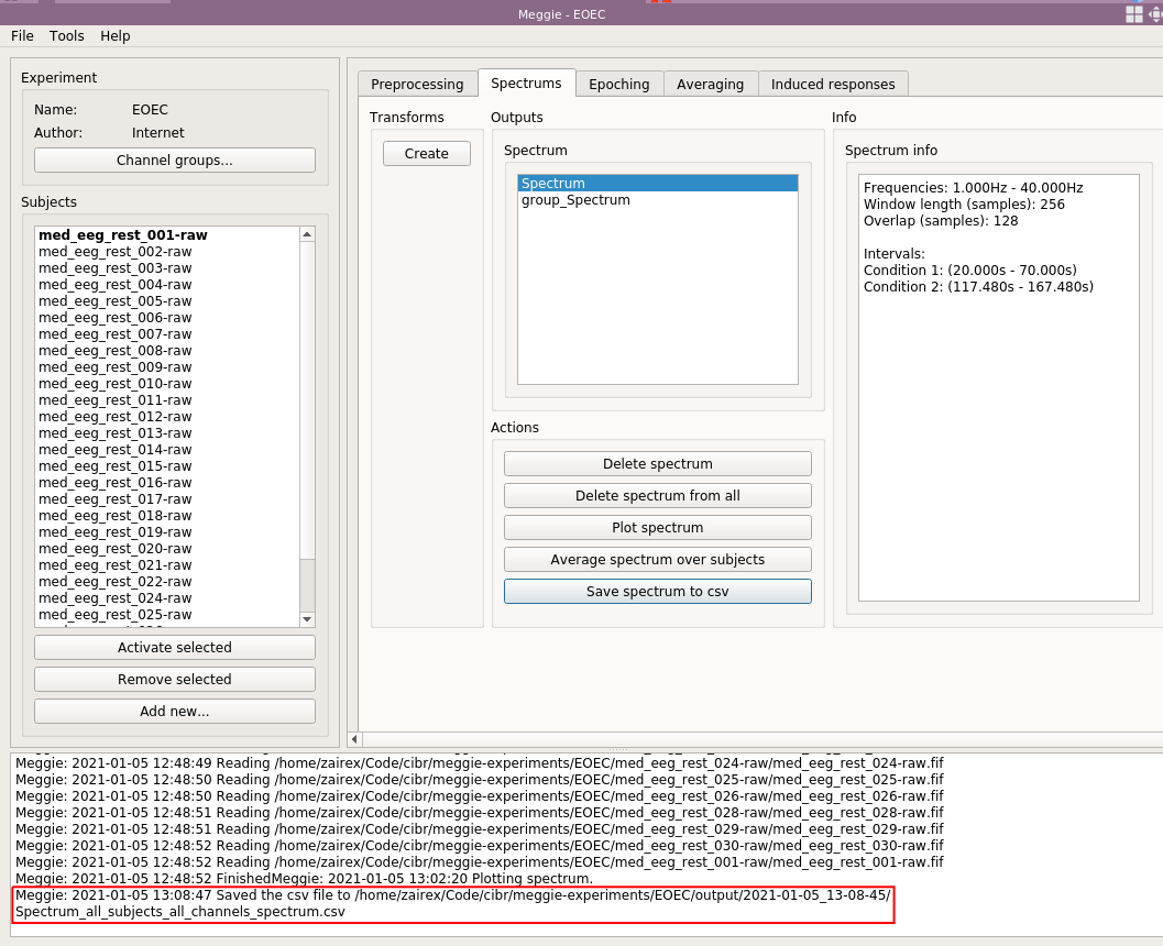
To finish, let us save the data for statistical analysis. Select the "Spectrum" item again, as we will want to save the data as it was before averaging over subjects, to, for example, do a standard t-test over subjects.

And click "Save spectrum to csv."

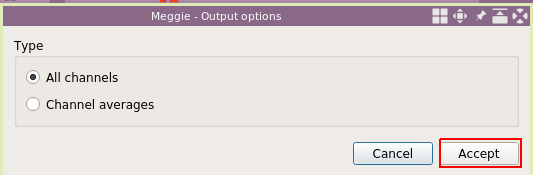
This time, keep "All channels selected" and click "Accept.". This will create one big csv file containing spectrums of all conditions and all channels and all subjects (spectrum items with the same name are looked under each subject).

The file is stored under experiment folder. The exact path is also printed to the console at the bottom of the screen.

The file opened using a standard spreadsheet program.